10.1 Introduction to irtools
A key part of the usualsuspects template is the use of Bayesian modeling for causal inferences.
The typical process is to model a dependent variable of interest (E.g. GPA) vs our treatment variable (E.g. participation in some program) while controlling for confounding (e.g. household income and/or race).
The brms package is used to set up these models and then several helper functions from the irtools package are used to clean up the results for printing.
10.1.1 Getting Started
First we need to load some of the required packages for our analysis.
10.1.2 Our Data
Again, we have simulated data for use.
This data is a part of the irtools package and is useful for demonstrating some of the available functionality in the package.
| ipeds_race | gender | student_ses | treated | gpa | hrs_earned | hrs_attempted | ap_hours_earned |
|---|---|---|---|---|---|---|---|
| Black | Female | Medium Income | 1 | 3.18 | 14.15 | 14.15 | 17.44 |
| Asian | Female | High Income | 1 | 3.00 | 13.43 | 13.43 | 17.76 |
| White | Female | Medium Income | 1 | 3.62 | 13.12 | 13.12 | 19.46 |
| NRA | Male | Low Income | 0 | 3.55 | 12.22 | 12.22 | 14.33 |
| White | Female | High Income | 0 | 3.68 | 11.45 | 11.45 | 12.83 |
| White | Male | High Income | 0 | 3.36 | 12.18 | 12.34 | 14.60 |
10.1.3 Fitting the Model
Say for example we want to test the effect of the treatment on a student’s gpa. We will also need to try to adjust the effect of our treatment by confounding factors (e.g. race and household income may have an impact on GPA).
We can build the model using the brm function from the brms package which has already been loaded as part of the irverse suite of packages.
First we generate the model that we want to fit. Here we are adjusting for race, gender, and student household income. The default is a normal distribution (i.e. a basic linear model. If this were binary response we would use a “bernouilli” distribution).
We can then fit this model.
As this is Bayesian modeling the Stan inference engine which powers the brms function can take some additional arguments to control how many iterations to run, how many chains to run and how to process these are your machine.
A ton of great documentation exists for brms and Stan.
If you want to learn more see the vignettes here and use the discussion board at the Stan website.
As with any R model we can look at the resulting parameters with the summary function.
##  Family: gaussian
##   Links: mu = identity; sigma = identity
## Formula: gpa ~ treated + gender + ipeds_race + student_ses
##    Data: fake_student_data (Number of observations: 500)
## Samples: 2 chains, each with iter = 1000; warmup = 500; thin = 1;
##          total post-warmup samples = 1000
##
## Population-Level Effects:
##                         Estimate Est.Error l-95% CI u-95% CI Eff.Sample
## Intercept                   3.20      0.04     3.12     3.28        389
## treated                     0.09      0.02     0.05     0.12       1419
## genderMale                 -0.01      0.02    -0.05     0.02       1020
## ipeds_raceBlack            -0.02      0.05    -0.11     0.09        469
## ipeds_raceHispanic         -0.02      0.05    -0.12     0.07        424
## ipeds_raceNAIA             -0.17      0.15    -0.46     0.14        938
## ipeds_raceNRA               0.00      0.05    -0.09     0.10        456
## ipeds_raceWhite             0.02      0.04    -0.06     0.09        336
## student_sesMediumIncome     0.03      0.03    -0.02     0.08       1160
## student_sesHighIncome       0.01      0.02    -0.03     0.05       1034
##                         Rhat
## Intercept               1.00
## treated                 1.00
## genderMale              1.00
## ipeds_raceBlack         1.00
## ipeds_raceHispanic      1.00
## ipeds_raceNAIA          1.00
## ipeds_raceNRA           1.00
## ipeds_raceWhite         1.00
## student_sesMediumIncome 1.00
## student_sesHighIncome   1.00
##
## Family Specific Parameters:
##       Estimate Est.Error l-95% CI u-95% CI Eff.Sample Rhat
## sigma     0.21      0.01     0.19     0.22       1094 1.00
##
## Samples were drawn using sampling(NUTS). For each parameter, Eff.Sample
## is a crude measure of effective sample size, and Rhat is the potential
## scale reduction factor on split chains (at convergence, Rhat = 1).
We can see from the Rhat diagnostics and Effective Sample sizes that we are achieving good convergences and can trust our results.
If we had more information to include in our priors we could include those in the brm model. See ?brm for more details.
10.1.4 Summarising the Results
Now we can use our helper functions from the irtools package to help summarise our results.
summarise_brms_results
We can use the summarise_brms_results function to pull out some summary information from our fitted model including the effect size, our point estimate for the effect as well as our credible interval.
Note that brms added a “b_” before our variable.
##        term   estimate  std.error      lower     upper     mu_gpa
## 1 b_treated 0.08582733 0.01893032 0.05511923 0.1165057 0.08582733
##     cohen_d      cles      type non_zero_effect Outcome
## 1 0.4140671 0.6605875 Cohen's D 1 gpa*make_standardized_betas
Note that the values from the summarise_brms_results are on the original scale (e.g. points on a 4.0 GPA scale).
However, when we are comparing across several different parameters sometimes we like to include standardized values in order to judge the order of magnitude (e.g. a 1pt GPA jump might be a bigger effect than a 1 hour move in credits earned). The make_standardized_betas function will standardize our coefficients.
## # A tibble: 1 x 4
##   std_beta_mu std_lower std_upper Outcome
##         <dbl>     <dbl>     <dbl> <chr>
## 1       0.201     0.129     0.273 gpa
Typically we want to look at these two tables together so we could easily combine them with:
##        term   estimate  std.error      lower     upper     mu_gpa
## 1 b_treated 0.08582733 0.01893032 0.05511923 0.1165057 0.08582733
##     cohen_d      cles      type non_zero_effect Outcome std_beta_mu
## 1 0.4140671 0.6605875 Cohen's D               1     gpa    0.201125
##   std_lower std_upper
## 1 0.1291646 0.2730157
10.1.5 Displaying the Outputs
The next step is to combine the results into the appropriate data frame structure.
It is important that certain column names exist in order to use the make_regression_results_graph.
These include those from the previously joined brms results as well as fields for
Pretty_Titlesignificantdescription
For example see below how I add them.
In the usualsuspects template most of this step is completely automated.
regression_fi <- combined_results %>%
  add_column(Pretty_Title = "Grade Point Average") %>%
  # Clean up and add some flags
  mutate_if(is.numeric, round, digits = 2) %>%
  left_join(outcome_description) %>%
  select(Pretty_Title, everything(), -Outcome) %>%
  mutate(significant = case_when(
    lower < 0 & upper < 0~ 1,
    lower > 0 & upper > 0 ~ 1,
    TRUE~ 0
  )) %>%
  mutate(description =ifelse(significant == 1, case_when(
    abs(cohen_d) < 0.05 ~ "Small",
    abs(cohen_d) >= 0.05 & abs(cohen_d) < 0.2~ "Medium",
    abs(cohen_d) >= 0.2 ~ "Large",
  ), "")) %>%
  make_regression_results_graph(treated_name = "Treated")
## Joining, by = c("Outcome", "Pretty_Title")Now we can use the make_tie_fighter_plot function to generate our familiar plot.
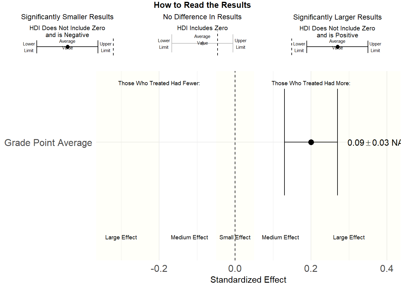
Figure 10.1: Regression Tie-Fighter Plot
This graph shows the standardized betas, uses the different criteria for effect size and includes the legend. If the initial table has more values (e.g. GPA, hrs earned, etc, this will automatically display them all together).